Nightlights

Those who follow the discussions about UHI understand that “nightlights” plays a large role in defining whether or not a station is considered Rural or Urban. In the work of GISS nightlights are determined by looking at the DSMP product. The product is available in 30 arcsecond format. That’s .00833 degrees. The following issue arises. The GHCN metadata is reported out at two resolutions: For the US,  the V3 inventory reports down to the 4th digit. X.yyyy. For the ROW the precision is X.yy. Further, we know that some of the locations are wrong. Herein lies the question. If you take the reading of nightlights from an aliased location or a faulty location, how good is your estimate?

I started out looking at this with raster. Of course I didnt read the manual entirely so I spent some time re inventing wheels. In the end I will illustrate two commands and how they help up start down the path to the answer:

url_radianceCalibrated<-"ftp://ftp.ngdc.noaa.gov/DMSP/web_data/rad_cal/rad_cal.tar"

calibratedLights<-"rad_cal.tar"

hiResTif<-"world_avg.tif"

download.file(url_radianceCalibrated,calibratedLights,mode="wb")

untar(calibratedLights)

gunZipDirectory(getwd())

hiResLights<-raster(hiResTif)

coords <-getInvLonLat(Inv)

cellId  <- cellFromXY(hiResLights,coords)

Lightc  <- cellValues(hiResLights,cells=cellId)

Inv <- cbind(Inv,DSMP=Lightc)

Inv <- cbind(Inv,Cell=cellId)

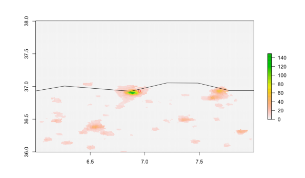
Very quickly. We download the lights file, untar it and then use a utility I wrote to ‘gunzip” the entire directory. Next we load the raster. It’s huge. Nightlights at 1km. Don’t even bother plotting it, you’ll see clouds of little points. Next, I pull out the cellId for every station. Then using those cells, I pull the value of nightlights at that location. Then I just add them to the inventory. To answer the question about the potential errors we need to look at the neighborhood. I tinkered around with calls to “adjacency” and “focal” but in the end settled on the following. First, extent:

e <- extent(6,8, 36.0, 38)

For this command I merely picked the coordinates of the first station: 6.95,36.95. I then bracket the lat and lon. Then we call ‘”crop”

r <-crop(hiResLights,e)

then plot:

plot(r)

points(36.93 6.95,col=’red’)

map(“world”,xlim=c(6,8),ylim=c(36,38),add=T)

later I’ll apply an SST mask, but this is what you see: