Modis QC Bits

In the course of working through my MODIS  LST project and reviewing the steps that Imhoff and Zhang took as well has the data preparations other researchers have taken ( Neteler ) the issue of MODIS Quality control bits came up.  Every MODIS  HDF file comes with multiple SDS or multiple layers of data. For MOD11A1 there are layers for daytime LST, Night LST, the time of  collection, the emissivity from ch 31 and 32,  and two layer for Quality Bits.  The various layers of   MODIS11A1  file is available here. Or if you are running the MODIS package, you can issue the getSds()  call and pass it the name of a HDF file.

As Neteler notes the final LST files contain pixels of various quality. Pixels that are obscured by clouds are not produced, of course, but that does not entail that every pixel in the map is of the same quality. The SDS layers for QC  — QC_day and QC_Night– contain the QC bits for every lat/lon  in the LST map. On the surface this seem pretty straighforward, but deciding the bits can be a bit of a challenge. To do that I considered several source.

 1. Neteler’s web post

2. The Modis groups  user guide

3. The  QA Tutorial

4. LP  DAAC  Tools, specifically the LDope tools provided by guys at MODLAN

I will start with 4, the ldope tools, If you are a hard core developer I think these tools would be a great addition to your bag of tricks. I won’t go into a lot of detail, but the tools allow you to do a host of processing on HDF files using a command line type interface. They provide source code in c and at some point in the future I expect that I would want to either write an R interface to these various tools  or take the C code directly and wrap it in R. Since they have the code for reading HDF directly and quickly it might be a source to use to support the direct import of HDF  into raster. However, I found nothing to really help with understanding the issue of decoding the  QC bits. You can manipulate the QC layer and do a  count of the various flags  in the data set. Using the following command on all the tiles for the US I was able to poke around and figure out what flags are typically reported

comp_sds_values -sds=QC_Day C:\\Users\\steve\\Documents\\MODIS_ARC\\MODIS\\MOD11A1.005\\2005.07.01\\MOD11A1.A2005182.h08v05.005.2008040085443.hdf

However,  I could do the same thing simply by loading a version of the whole US into raster and using the freq() command on raster. Figuring about what values are in the QC file is easy, but we want to understand what they mean. Let’s begin with that list of values. By looking at the frequency count of the US raster and by looking at a large collection of HDf files I found the following values for the QC layer

values <-c(0,2,3,5,17,21,65,69,81,85,129,133,145,149,193)

The question is  what do they mean. The easiest one to understand is 0. A zero means that this pixel is highest quality. If we want only the highest quality pixels, then we can use the QC map, turn it into a logical mask and apply it to the  LST map such that we only keep pixels that  have 0 for their quality bits. There, job done!

Not so fast. We throw away many good pixels that way. To understand the QC bits lets start with the table provided

If you are not clear on how  this works  every number, every integer in the QC map is an unsigned 8 bit integer. The range of numbers is 0 to 255. The integers represent bit codes which requires you to do some base 2 math. That is not the tricky part. The number 8 for example would be   “0001”  and 9 would be  1001.  If you are unclear about binary representations of integers I suppose google is your friend.

Given the binary representation of the integer value we are then in a position to understand what the quality bits  represent, but there is a minor complication which I’ll explain using an example.  Let’s take  the integer value of 65.  In R the way we turn this into a binary representation is by using the call intToBits.

intToBits(65)
[1] 01 00 00 00 00 00 01 00 00 00 00 00 00 00 00 00 00 00 00 00 00 00 00 00
[25] 00 00 00 00 00 00 00 00

We only need 8 bits, so we should do the following

> intToBits(65)[1:8]
[1] 01 00 00 00 00 00 01 00

and for more clarity I will turn this into 0 and 1 like so

> as.integer(intToBits(65)[1:8])
[1] 1 0 0 0 0 0 1 0

So the first bit ( or bit 0 ) has a value of 1, and seventh bit  ( bit 6 ) has a value of 1.  We can check our math 2^6 =64  and 2^0 = 1, so it checks. Don’t forget that the 8 bits are numbered 0 to 7 and each represents a power of 2.

If you try to use this bit representation to understand the  QC “state”,  you will go horribly wrong!. It’s wrong because HDF files are written in big endian format. If you are not familiar with that, what you need to understand is that the least significant bit is on the right. In the example above the zero bit is on the left, so we need to flip the bits so that bit zero is on the right . Little Endian goes from right to left, 2^0 to 2^7. Big Endian goes left to right 2^7 to 2^0.

Little Endian:   1 0 0 0 0 0 1 0   = 65       2^0 + 2^6

Big Endian  0 1 0 0 0 0 0 1         = 65        2^6 + 2^0

The difference is this:

If we took  1 0 0 0 0 0 1 0 and ran it through the table, the table would indicate that  the first two bits 10  would mean the pixel was not generated, and  bit 1 in the 6th position would indicate an LST error of  <= 3K.  Now flip those bits

> f<-as.integer(intToBits(65)[1:8])
> f[8:1]
[1] 0 1 0 0 0 0 0 1

This bit order has the first two bits as 01 which indicates that the pixel is produced, but that other quality bits should be checked. Since bit 6 is 1 that indicates  the pixel has an error > 2Kelvin but less than 3K

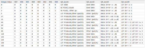
In short,  to understand the QC bits we first turn the integer into a bit notation and then we flip the order of the bits and then use the table to figure out the QC status.  For MOD11A1 I wrote a quick little program to generate all the possible bits and then  add descriptive fields. I would probably do this for every Modis project I worked on especially since I dont work in binary everyday and I made about 100 mistakes trying to do this in my head.

QC_Data <- data.frame(Integer_Value = 0:255,
Bit7 = NA,
Bit6 = NA,
Bit5 = NA,
Bit4 = NA,
Bit3 = NA,
Bit2 = NA,
Bit1 = NA,
Bit0 = NA,
QA_word1 = NA,
QA_word2 = NA,
QA_word3 = NA,
QA_word4 = NA
)

for(i in QC_Data$Integer_Value){
AsInt <- as.integer(intToBits(i)[1:8])
QC_Data[i+1,2:9]<- AsInt[8:1]
}

QC_Data$QA_word1[QC_Data$Bit1 == 0 & QC_Data$Bit0==0] <- “LST GOOD”
QC_Data$QA_word1[QC_Data$Bit1 == 0 & QC_Data$Bit0==1] <- “LST Produced,Other Quality”
QC_Data$QA_word1[QC_Data$Bit1 == 1 & QC_Data$Bit0==0] <- “No Pixel,clouds”
QC_Data$QA_word1[QC_Data$Bit1 == 1 & QC_Data$Bit0==1] <- “No Pixel, Other QA”

QC_Data$QA_word2[QC_Data$Bit3 == 0 & QC_Data$Bit2==0] <- “Good Data”
QC_Data$QA_word2[QC_Data$Bit3 == 0 & QC_Data$Bit2==1] <- “Other Quality”
QC_Data$QA_word2[QC_Data$Bit3 == 1 & QC_Data$Bit2==0] <- “TBD”
QC_Data$QA_word2[QC_Data$Bit3 == 1 & QC_Data$Bit2==1] <- “TBD”

QC_Data$QA_word3[QC_Data$Bit5 == 0 & QC_Data$Bit4==0] <- “Emiss Error <= .01”
QC_Data$QA_word3[QC_Data$Bit5 == 0 & QC_Data$Bit4==1] <- “Emiss Err >.01 <=.02”
QC_Data$QA_word3[QC_Data$Bit5 == 1 & QC_Data$Bit4==0] <- “Emiss Err >.02 <=.04”
QC_Data$QA_word3[QC_Data$Bit5 == 1 & QC_Data$Bit4==1] <- “Emiss Err > .04”

QC_Data$QA_word4[QC_Data$Bit7 == 0 & QC_Data$Bit6==0] <- “LST Err <= 1”
QC_Data$QA_word4[QC_Data$Bit7 == 0 & QC_Data$Bit6==1] <- “LST Err > 2 LST Err <= 3”
QC_Data$QA_word4[QC_Data$Bit7 == 1 & QC_Data$Bit6==0] <- “LST Err > 1 LST Err <= 2”
QC_Data$QA_word4[QC_Data$Bit7 == 1 & QC_Data$Bit6==1] <- “LST Err > 4”

Which  looks like this

Next,  I will remove those flags that don’t matter.  All good pixels, all pixels that don’t get drawn, and  those where the TBD bit is set high. What I want to do is select all those flags where the pixel is produced but the pxel quality is not the highest quality

FINAL <- QC_Data[QC_Data$Bit1 == 0 & QC_Data$Bit0 ==1 & QC_Data$Bit3 !=1,].  Below see a part of this table

And then I can select those  that occur in my HDF files.

Looking at LST error which matters most to me, the table indicates that I can use pixels that have a  QC value of 0,5,17 and 21. I want to only select  pixels where LSt error is less than 1 K

Very quickly I’ll show how one uses raster functions to apply the QC bits to  LST.   using MODIS R and the function  getHdf() I’ve downloaded all the tiles for US for every day in July 2005. For July 1st, I’ve used  MRT to mosiac and resample  all the SDS. I use Nearest neighbor to insure that I dont average quality bits. The mosaic is the projected from a SIN projection to a Geographic projection ( WGS84) and a geotiff output format. Pixel size is set at   30 arc seconds

The SDS are read in using R’s raster

library(raster)

##  get every layer of data in the July1 directory

SDS <- list.files(choose.dir(),full.names=T)

##  for now I just work with the Day data

DayLst <- raster(SDS[7])
DayQC <- raster(SDS[11])

##  The fill value for LST is Zero. That means Zero represents a No Data pixel

##  So, we force those pixels to NA

DayLst[DayLst==0]<-NA
NightLst[NightLst==0]<-NA

##  Units in LST  need to be scaled to be put into Kelvin. The adjustment value is  .02.  See the docs for these values

##  every SDS has a different fill value and a different scaling value.
DayLst <- DayLst * .02

Now, we can plot the two raster

plot(DayLst, main = “July1 2005 Day”)

plot(DayQC, main=”Day Quality COntrol”)

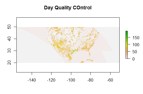
And I note  that the area around texas has a nice variety of QC bits, so we can zoom in on that

Next we will use  the QC  layer and create mask

m <- DayQC
m[m > 21]<-NA
m[ m == 2 | m== 3]<-NA

Good <- mask(DayLst, m)

For this mask I’ve set all those grids with  QC bits  greater than 21 to NA.  I’ve also set  QC pixels with a value of 2 and 3 to NA.  This step isnt really necessary  since  QC  values of 2 and 3 mean that the pixel doesnt get produce, but I want to draw a map of the mask which will show which bits are NA and which bits are not NA.  The mask() function works like so. “m” is laid over DayLst.  bits that are NA in “m” will be NA in the destination (“Good”)  if a pixel is not NA in “m” and has a value like, 0 or 17 or 25, then the value of the source (DayLst) is written into the destination.

Here are the values in my mask

> freq(m)
value    count
[1,] 0        255179
[2,] 5         12
[3,] 17       8539
[4,] 21        3
[5,] NA   189147

So the mask will “block” 189147 pixels in DayLst from being copied from source to destination, while allowing the source pixels that have QC bits of 0,5,17,21 to be written. These QC bits  are those that represent an LST error of less than 1K

When this mask is applied the colored pixels will be replaced by the values in the “source”

And to recall, these are all the pixels PRIOR to the application of the QC bits

As a side note, one thing I noticed when doing my SUHI analysis was that the LST data had a large variance over small areas. Even when I normalized for elevation and slope and land class there were  pixels that were 10+ Kelvin warmer than the means. Essentially 6 sigma cases. That, of course lead me to have a look at the QC bits.  Hopefully, this will improve some of the R^2 I was getting in my test regressions.

Modis R: Package tutorial

The MODIS package for R

For people who work in GIS in R there has been a bit of challenge in working with data from  Modis. I’ll use an example from my own work on UHI to illustrate. A while back I decided that I wanted to look at albedo data from MODIS.  If you want to get MODIS data there are basically two approaches. You can use  the web services  like REVERB which is basically a web interface that allows you to construct queries for a wide variety of data ( or similar services shown here ) or you can download files directly from the datapool ftp.

For my Albedo project I decided to download directly from ftp because I could write a simple program in R to collect the entries in the ftp directories and then download them over the course of a few hours.  It’s essentially the same process I use in my study of SUHI for small cities. Getting the data locally is not a big problem, except for the storage issue.  You can imagine what it would take to download 90 days of LST data for the US.  with 10-14 tiles of data required that ends up being a nice chunk of data.

The next challenge is getting MODIS data out of its native format into a format that is friend for R GIS packages. In the case of Albedo that data was stored in a format known as “HDF” or HDF-EOS.  I work with  the raster package and raster ( along with rgdal)  have no way of reading HDF directly. This meant I had to find a way to transform HDF into a more common format like “geoTiff”. There was also the issue of tiling multiple hdf files into a single raster. Unlike other datasets that might give you a monolithic file of the whole world, the MODIS collections are distributed as tiles using their tiling system.

To solve this problem there are a couple tools: MRT or the modis reprojection tool. or GDAL, the Geospatial Data abstraction Library. For Albedo I decided to use GDAL and I used the distribution of GDAL provided by FWTools.  With a few hundred albedo files I had to write a script to load every Hdf file and transform it to a ‘geotiff’ file. That worked fine, but now I had a set of R code for doing my statistics and a “bat” file for controlling Gdal.  With my SUHI project I decided to use MRT. In that case I used the GUI they provide to select all the files, mosaic them, crop them, resample and reproject. I quickly learned that duplicating the same steps with a GUI is not always easy. Further, if I am trying to create work that is reproduceable, it makes it hard. Plus I could not see using that tool to create 365 maps for every day in the year.

What’s needed is an R package that allows us to write R code and achieve the same results as we get with GDAL or MRT. We want to write R code that controls these external applications and tools. That’s what  MODIS R does.

The team: The MODIS R team consists of  Matteo Mattiuzzi, Jan Verbesselt, Forrest Stevens, Tomislav Hengl, Anja Klisch, Bradley Evans and Agustin Lobo. Some of the seminal work was done by Tomislav at his wonderful page

My Tutorial.  I had some discussions with Matteo who is the package maintainer and  suggested that I might do a tutorial to help people get started with the package.  At this stage the package is stable, so I decided to start a tutorial. The way I work is pretty simple. As I try  new things I write them up.    For now the tutorial  starts with the basics of R, R studio and preparing your system for MODIS R. That includes downloading a the tools and testing them out and finally downloading and building a WINDOWS version of MODIS R.

Then I will start to go through the API and test and explain all the calls in more depth than the manual and write some sample code.

A note. If you have questions about what I am doing go ahead and leave comments. I can collect up questions and those I cant answer I can pass on to the maintainers.

The tutorial starts here

More Fun With Modis

I’ve started a tutorial on using the MODIS package in R the first few steps are here.  While I wait on a release of the package I thought I would play around a bit with the MRT tool and see how it worked.  Let’s recall where we are going.  I have an inventory of around 150 small cities and we are going to take a look at SUHI in those locations.  I have the DEM data, The Modis Land Class data, Olson Biomes, NLCD 30 meter land class and impervious surface. The last few bits I will need are MODIS LST and perhaps MODIS albedo ( If I get motivated) and EVI. We also have population data from a couple sources and housing data.

The first step to getting MODIS LST data is deciding what Tiles I need and then selecting dates. I had hoped that I might get away with using just a few tiles for the US, but that doesnt look like its going to happen. To figure out which Tiles I need there is a function in the MODIS package called getTile. But before I figured that out I tried to do it on my own. With some help from the geo sig list  I have the following to figure out the tiles.

First I get the  bounding coordinates for every tile

library(geosphere)

library(sp)

gring <-“http://landweb.nascom.nasa.gov/developers/sn_tiles/sn_gring_10deg.txt&#8221;

 
GRING <- read.table(gring, skip = 7, stringsAsFactors =FALSE, nrows=648,
na.strings=c(“-999.0000″,”-99.0000″))

colnames(GRING)<-c(“v”,”h”,”ll_lon”,”ll_lat”,
“ul_lon”,”ul_lat”,”ur_lon”,”ur_lat”,
“lr_lon”,”lr_lat”)

GRING <- GRING[!is.na(GRING[,3]),]

DF <- GRING[GRING$h < 15 & GRING$h > 6 & GRING$v < 7 & GRING$v > 3,]

The  table is downloaded and then I remove those rows that are NA. Next, I select those parts of the table that relate to CONUS  between  h(horizontal) 15 and 6 and vertical 7 and 3.

Next, I use Robert Hijmans code for generating a spatialpolygondataframe.

m <- as.matrix(DF)
z <- apply(m, 1, function(x) Polygon(matrix(x[c(3:10, 3:4)], ncol=2, byrow=T)))
n <- names(z)
y <- sapply(1:length(n), function(i) Polygons(z[i], n[i]))
sp <- SpatialPolygons(y, proj4string=CRS(‘+proj=longlat’))
spdf <- SpatialPolygonsDataFrame(sp, DF)

then we make some corrections for being on a sphere and we read in the lat/lon of all 150 sites
spdfc <- makePoly(spdf)

Inv <- read.table(“SiteInventory.inv”,stringsAsFactors = FALSE)

The next bit of clumsy code creates a spatial points data frame  that has 4 points for every site. I’m going to look +- .5degrees from the site center.

myExtent <- data.frame(lon=rep(NA,4*nrow(Inv)),lat=rep(NA,4*nrow(Inv)))

for( site in 1:nrow(Inv)){
dex <- ((site-1)*4)+1
myExtent$lon[dex]<- Inv$Lon[site] +.5
myExtent$lat[dex]<- Inv$Lat[site] -.5
myExtent$lon[dex+1]<- Inv$Lon[site] +.5
myExtent$lat[dex+1]<- Inv$Lat[site] +.5
myExtent$lon[dex+2]<- Inv$Lon[site] -.5
myExtent$lat[dex+2]<- Inv$Lat[site] -.5
myExtent$lon[dex+3]<- Inv$Lon[site] -.5
myExtent$lat[dex+3]<- Inv$Lat[site] +.5

}

Finally we will intersect the points with the SpatialPolygonsDataframe  and get out the tiles

pts <- SpatialPoints(myExtent)

proj4string(pts)<- proj4string(spdf)

Tiles <- over(pts,spdfc)[1:2]

Tiles <- unique(Tiles)

nrow( Tiles)

print(Tiles)

Depending on the increment I used  (.5 versus .2)  I basically had to collect 10-12 tiles to cover my bases for the next step.

With that list of tiles I downloaded the tiles I needed for  July4th  2006. In the future with the MODIS package this will happen just by writing code, but for now I did it by hand. With those 12 tiles downloaded I then fired up MRT to mosaic , resample, and reproject the tiles into a monolithic GeoTiff  for daytime LST for the whole Conus.

Reading that it we get the following

And then we can zoom in on the midwest and then go down chicago

On the left at  lon -87.9 lat 41.65  is the Paw Paw Woods Nature Preserve.  Pretty Cool